We use cookies on this website to distinguish you from other users. We use this data to improve our content experience and for targeted advertising. By continuing to use this website you consent to our use of cookies. For more information, please see our Cookie Policy.

spafe.frequencies.fundamental_frequencies#

Description : Implementation Fundamental Frequency Extraction Using the YIN-Algorithm.
Copyright (c) 2019-2023 Ayoub Malek. This source code is licensed under the terms of the BSD 3-Clause License. For a copy, see <https://github.com/SuperKogito/spafe/blob/master/LICENSE>.

spafe.frequencies.fundamental_frequencies.compute_difference(x: ndarray, tau_max: int) → ndarray[source]#

Compute difference function of data x according to [Guyot] [DeCheveigné] and [Box] . This essentially corresponds to equations (6) and (7) in [DeCheveigné]

Parameters

x (numpy.ndarray) – audio array data.
tau_max (int) – integration window size.

Returns

difference function resulting array.

Return type

(numpy.ndarray)

Note

\[ \begin{align}\begin{aligned}d_{t}(\tau) = \sum_{j=1}^{W}(x_{j} - x_{j+\tau})^{2}\\d_{t}(\tau) = r_{t}(0) + r_{t+\tau}(0) - 2 r_{t}(\tau)\end{aligned}\end{align} \]

where \(d_{t}(\tau)\) is the difference function, \(r_{t}(\tau)\) is the autocorrelation.

This function use an accellerated convolution function fftconvolve from the Scipy package to compute the autocorrelation for faster processing.
While the brute force algorithm time complexity is O(n**2), the Wiener–Khinchin theorem allows computing the autocorrelation with two Fast Fourier transforms (FFT), with time complexity O(n log(n)).
The steps for computing the autocorrelation according the Wiener–Khinchin theorem are as follows:
\[ \begin{align}\begin{aligned}F_{R}(f) = FFT[X(t)]\\S(f) = F_{R}(f) + F^{*}_{R}(f)\\R(\tau) = IFFT[S(f)]\end{aligned}\end{align} \]

where IFFT is the inverse fast Fourier transform and the asterisk denotes complex conjugate.

References

Box: : Box, G. E. P., Jenkins, G. M., Reinsel, G. C. (1994). Time Series Analysis: Forecasting and Control (3rd ed.). Upper Saddle River, NJ: Prentice–Hall. ISBN 978-0130607744.

spafe.frequencies.fundamental_frequencies.compute_cmnd(d_t: ndarray, tau: int) → ndarray[source]#

Apply Cumulative Mean Normalized Difference Function (CMNDF) as in [Guyot] [DeCheveigné]. This corresponds to equation (8) in [DeCheveigné].

Parameters

d_t (numpy.ndarray) – Difference function array.
tau (int) – length of data.

Returns

cumulative mean normalized difference

Return type

(numpy.ndarray)

Note

\[\begin{split}d^{\prime}_{t}(\tau)=\left\{\begin{array}{l} 1, & \text{if } \tau = 0 \\ \frac{d_{t}(\tau)}{\frac{1}{\tau} \sum_{j=1}^{\tau} d_{t}(j)}, & \text{otherwise } \end{array}\right.\end{split}\]

spafe.frequencies.fundamental_frequencies.get_pitch(cmdf: ndarray, tau_min: int, tau_max: int, harmonic_threshold: float = 0.1) → float[source]#

Return fundamental period of a frame based on CMND function as implemented in [Guyot] [DeCheveigné].

Parameters

cmdf (numpy.ndarray) – cumulative mean normalized difference
tau_min (int) – minimum period for speech.
tau_max (int) – maximum period for speech.
harmonic_threshold (float) – harmonicity threshold to determine if it is necessary to compute pitch frequency. (Default is 0.1).

Returns

fundamental period if there is values under threshold, 0 otherwise

Return type

(float)

spafe.frequencies.fundamental_frequencies.compute_yin(sig: ndarray, fs: int, win_len: float = 0.03, win_hop: float = 0.015, low_freq: float = 50, high_freq: float = 3000, harmonic_threshold: float = 0.1) → Tuple[ndarray, ndarray, ndarray, ndarray][source]#

Compute the fundamental frequency and harmonic rate according to the the Yin Algorithm [Guyot] [DeCheveigné].

Parameters

sig (numpy.ndarray) – audio signal (list of float)
fs (int) – sampling rate (= average number of samples pro 1 second)
win_len (float) – size of the analysis window (in seconds) (Default is 0.03).
win_hop (float) – size of the lag between two consecutives windows (in seconds) (Default is 0.015).
low_freq (float) – Minimum fundamental frequency that can be detected (in Hertz) (Default is 50).
high_freq (float) – Maximum fundamental frequency that can be detected (in Hertz) (Default is 3000).
harmonic_threshold (float) – Threshold of detection. The yalgorithmù return the first minimum of the CMND fubction below this threshold. (Default is 0.1).

Returns

tuple include the following

pitches (numpy.array) : list of fundamental frequencies.
harmonic_rates (numpy.array)list of harmonic rate values for each fundamental
frequency value (= confidence value).
argmins (numpy.array) : minimums of the Cumulative Mean Normalized DifferenceFunction.
times (numpy.array) : list of time of each estimation.

Return type

(tuple)

References

DeCheveigné(1,2,3,4,5,6): : De Cheveigné, A., & Kawahara, H. (2002). YIN, a fundamental frequency estimator for speech and music. The Journal of the Acoustical Society of America, 111(4), 1917-1930.
Guyot(1,2,3,4): : Guyot, P. (2018, April 19). Fast Python implementation of the Yin algorithm (Version v1.1.1). Zenodo. http://doi.org/10.5281/zenodo.1220947

Examples

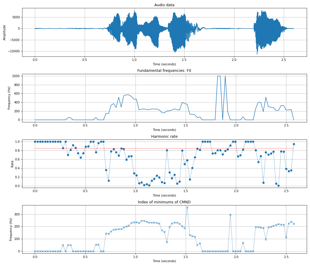
from scipy.io.wavfile import read
from spafe.frequencies.fundamental_frequencies import compute_yin


# read audio
fpath = "../../../tests/data/test.wav"
fs, sig = read(fpath)
duration = len(sig) / fs
harmonic_threshold = 0.85

pitches, harmonic_rates, argmins, times = compute_yin(sig,
                                                      fs,
                                                      win_len=0.050,
                                                      win_hop=0.025,
                                                      low_freq=50,
                                                      high_freq=1000,
                                                      harmonic_threshold=harmonic_threshold)

# xaxis helper function
gen_xaxis_times = lambda v, dt : [float(x) * dt / len(v) for x in range(0, len(v))]


plt.figure(figsize=(14, 12))
plt.subplots_adjust(left=0.125, right=0.9, bottom=0.125, top=0.9, wspace=0.2, hspace=0.99)

# plot audio data
ax1 = plt.subplot(4, 1, 1)
ax1.plot(gen_xaxis_times(sig, duration), sig)
ax1.set_title("Audio data")
ax1.set_ylabel("Amplitude")
ax1.set_xlabel("Time (seconds)")
plt.grid()

# plot F0
ax2 = plt.subplot(4, 1, 2)
ax2.plot(gen_xaxis_times(pitches, duration), pitches)
ax2.set_title("Fundamental frequencies: F0")
ax2.set_ylabel("Frequency (Hz)")
ax2.set_xlabel("Time (seconds)")
plt.grid()

# plot Harmonic rate
ax3 = plt.subplot(4, 1, 3, sharex=ax2)
ax3.plot(gen_xaxis_times(harmonic_rates, duration), harmonic_rates, ":o")
ax3.plot(gen_xaxis_times(harmonic_rates, duration), [harmonic_threshold] * len(harmonic_rates), "r:")
ax3.set_title("Harmonic rate")
ax3.set_ylabel("Rate")
ax3.set_xlabel("Time (seconds)")
plt.grid()

# plot Index of minimums of CMND
ax4 = plt.subplot(4, 1, 4, sharex=ax2)
ax4.plot(gen_xaxis_times(argmins, duration), argmins, ":x")
ax4.set_title("Index of minimums of CMND")
ax4.set_ylabel("Frequency (Hz)")
ax4.set_xlabel("Time (seconds)")
plt.grid()
plt.show()

../_images/fundamental_frequencies-1.png

spafe.frequencies.dominant_frequencies

spafe.utils